To make quantum computers, you need to know a lot about quantum physics. But to use them, you don't need to know all that. With this introduction, you will be able to model quantum computations by creating a simple quantum simulator with a few lines of code, as detailed in an appendix.
This primer is based on the book Building Quantum Software with Python (also available on Amazon). The accompanying code repositories are available on GitHub: code (Python) and code_js (JavaScript).
When explaining new ideas, it's helpful to start with what people already know. But what common knowledge is useful in learning quantum computing? Many think you need to study high-level linear algebra before understanding quantum computing's strange nature. This isn't true. Basic math (like binary numbers, trigonometry, and probabilities) is enough.
Quantum computers have two main features that regular computers don't: quantum parallelism and quantum measurement. Classical computers have limited ways of parallel computing (like vector processing and SIMD), which are like quantum parallelism, but only on a small scale. They can also take samples from probability distributions, similar to quantum measurement, but again, they can only do this efficiently on a small scale.
It turns out that using simple math not only simplifies understanding but also enhances performance when modeling quantum computations.
You're used to using numbers to understand systems that matter to you, like the stuff in your fridge, your account balances, or your investment portfolio. In portfolios, percentages have to add up to 100, and you can change your allocations by moving money between investments.
Quantum systems also have attributes with values that are constrained as a total, and you can change them with quantum transformations, which essentially move values between attributes.
The big difference is what happens when we observe (measure) a quantum system's state. The system's state collapses into one with just one attribute, like putting all your investments into one instrument. We only see one attribute at random, with a likelihood that depends on its value. This is the only strange thing about quantum systems, but once you understand it, it is not hard to use it.
Philosophers of science often engage in discussions about the existence of these values prior to observation. When it comes to designing quantum programs, these values are relevant, as they must be taken into consideration. Therefore, from the perspective of quantum program developers, these values are considered to exist. However, they are not stored anywhere, like we are used to values in classical computing. They are similar to attributes like the speed or the rotations per minute desribing the state of a car. We know how to change and measure them without directly writing and reading them.
In a quantum computation, the state of the underlying quantum system is altered, and there are various possible outcomes, each with a particular probability. These potential outcomes are attributes of the quantum system's state.
When executing a quantum program on a quantum computer, a single outcome is observed upon measuring the state of the quantum system. To obtain valuable information, the same program must be run multiple times, and the results of each run must be collected. A single execution is commonly referred to as a shot, while the number of times an outcome is observed is called a count.
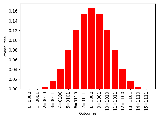
The behavior of a quantum program, when observed multiple times, is analogous to a Galton board, also known as a bean machine. This device consists of a vertical board with rows of pegs that are alternately positioned. Beads dropped from the top of the board bounce left or right as they encounter the pegs, ultimately landing in bins at the bottom. The resulting distribution of accumulated bead columns in these bins closely resembles a bell curve. By adjusting the arrangement of the pegs, one can generate different probability distributions.
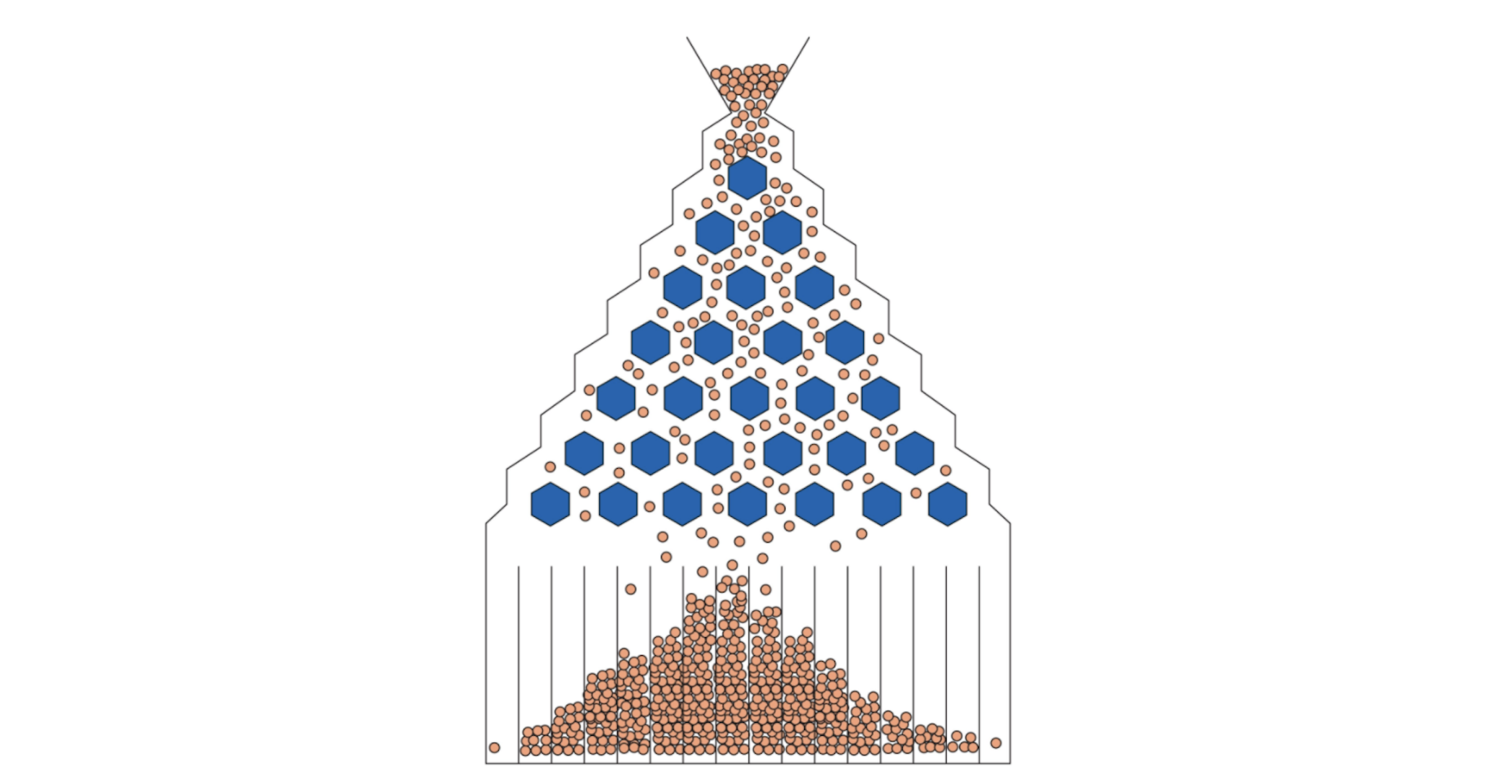
By converting the counts into percentages of the total number of runs, a probability histogram can be created, with each outcome being assigned a percentage based on its count, sometimes called a quasi-probability.
While we can only count outcomes of a quantum computation and approximate their probabilities, the values comprising a quantum state (one per possible outcome) are not straight probabilities. They are complex numbers, called probability amplitudes, or simply amplitudes. We can think of an amplitude as an arrow, or force, having a magnitude and a direction. The probability of an outcome is actually the squared magnitude of its amplitude. This is one of the fundamental facts of quantum theory that we just accept without trying to explain.
Depending on the context, it is useful to visualize an amplitude (complex number) in two ways:
1. An arrow starting from the origin of the plane and pointing to the corresponding point of the complex number.
2. A colored bar with a length equal to the magnitude (absolute value) of the complex number, and a color determined by the phase (direction) of the complex number, as depicted on the color wheel below.
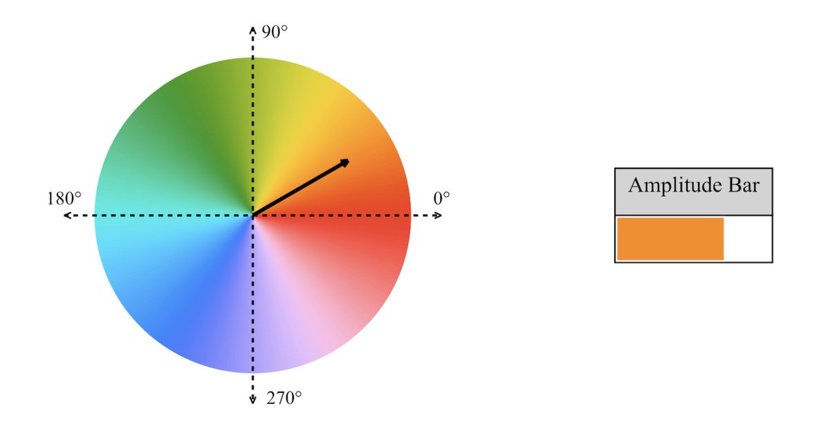
The amplitudes comprising the state of a qubit system cannot have magnitudes larger than 1, since the squared magnitudes are probabilities.
This is the most advanced math needed in this article. Recall that a complex number has an algebraic form:
and a polar form
Where \( i \) is the imaginary unit, with the property
A complex number corresponds to a point in the plane.
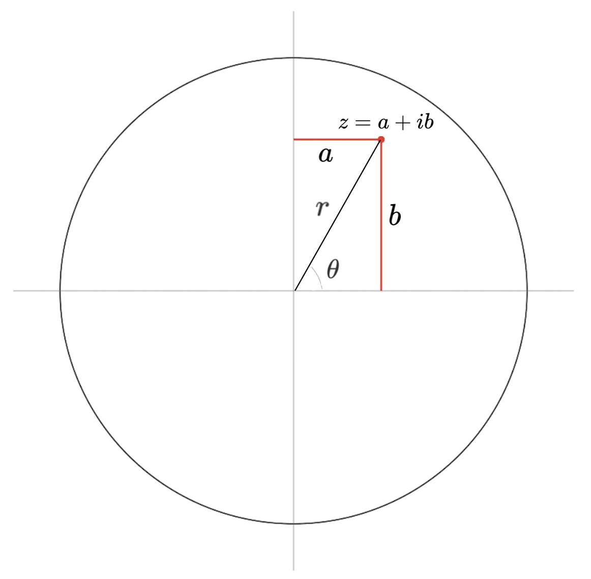
We can convert from the algebraic to the polar using simple formulas:
As mentioned, each possible outcome of a quantum computation has a probability amplitude associated to it, and the probability of an outcome is the squared magnitude of its corresponding amplitude. The sum of the probabilities of all possible outcomes adds up to 1.
We can use table "comprehensions" (term borrowed from Python's list comprehensions) to visualize quantum states algebraically.

Such a comprehension table can be seen as a bridge between formal math and code. Python code to express the same state looks like this:
state = [a[k] + 1j * b[k] for k in range(N)]
You don't need to understand the following formula, but this is how a quantum state is typically expressed mathematically:
In our experience, using tables is very effective in expressing quantum states, for all audiences.
We can use the polar form in tables as well:

It's sometimes useful to include more information in table rows, to get a deeper understanding of a quantum state:

Comprehension tables are used to show formulas or expressions in quantum states. For a concrete state, we can use a state table with one row of expanded information for each possible outcome of a quantum computation, or a simpler polar area diagram where the outcomes are represented by circle sectors, and their probabilities are sub-sectors whose area is proportional to the probability.
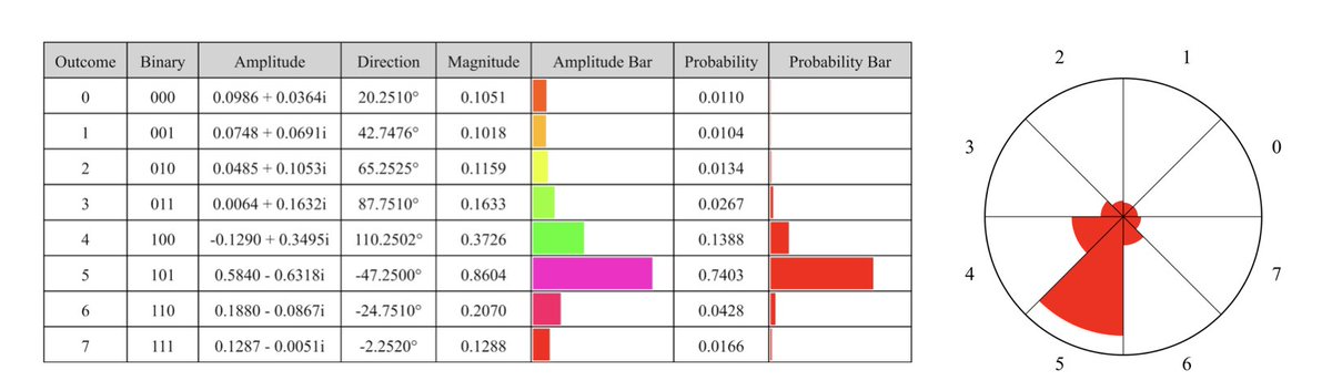
These two representations are versions of a bar plot and can be preferred in different contexts.
A qubit is a digit in the binary representation of outcomes. A quantum system with a single qubit has two possible outcomes, 0 or 1. A two-qubit system has four possible outcomes, consisting of all two-digit binary numbers:
Similarly, a three-qubit system has eight possible outcomes, consisting of all three-digit binary numbers:
In general, an \(n\)-qubit quantum system supports quantum computations with:
outcomes.
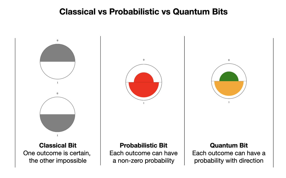
How do we explain the difference between a classical and a quantum bit? A quantum bit, or better said, a one-qubit system, has a probability with direction for each of the two possible outcomes, while in a classical bit, exactly one outcome is possible. We represent outcomes with circle sectors, and directions with colors on a color wheel. For two outcomes, the sectors are semi-circles. Note that the comparison works only for one-(qu)bit systems, not for a (qu)bit in a larger system. Many comparisons in the quantum computing literature are incorrect or incomplete, especially those saying that a qubit can have any value between 0 and 1.
We visualize the effect of applying quantum gates using table comprehensions, state tables, and color wheels.
The X-gate, also called the NOT gate, swaps the amplitudes corresponding to a pair of outcomes.
How to use this app: Select a gate, target qubit, and (if needed) a control qubit using the controls above the visualizer. Click 'Start Transformation' to begin the process - this will highlight the first pair of amplitudes that will be transformed. The pairs represent outcomes whose binary representations differ only in the target qubit position. For controlled gates, only pairs where the control qubit is 1 will be processed. Use 'Process Next Pair' to transform one pair at a time, or 'Process All Pairs' to complete the transformation at once. 'Reset' returns to the default state, and 'Randomize' creates a new random state. You can experiment with different gates and qubit choices to see their effects on the quantum state.
Try with target qubits 0, 1, and 2:
Applying a Y-gate to a single-qubit state changes both the directions and swaps the probabilities, as shown in the diagram.
This gate multiplies the 1-side of a pair of amplitudes by -1. It changes the signs of both the real and imaginary parts of the amplitude of the 1-side of the pair.
The Hadamard gate (or H-gate), named after the famous mathematician Jacques Hadamard, replaces an amplitude pair with their sum and difference divided by the square root of 2.
The Phase gate rotates the 1-side of a pair of amplitudes by a given angle.
For a given angle θ, the RZ(θ)-gate rotates the 0-side of a pair of amplitudes counterclockwise by θ/2, and the 1-side of a pair of amplitudes clockwise by θ/2.
An elementary quantum transformation is a single-qubit gate applied to a target qubit.
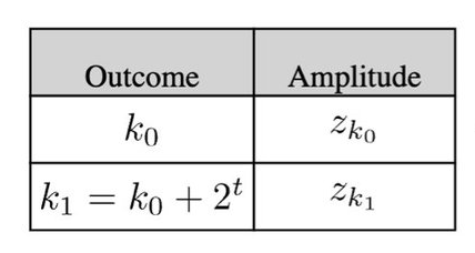
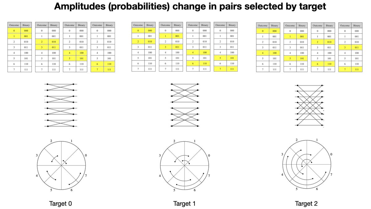
We can visualize and explain quantum state evolution with elementary quantum gates using the important, but often ignored fact that amplitudes change in pairs, with the pairing depending on the target of a gate application. If the target qubit is t, two outcomes are paired if their binary representation differ only in the digit t. This means that their difference is
We can represent the pairing of outcomes and amplitudes with two generic rows in a table:
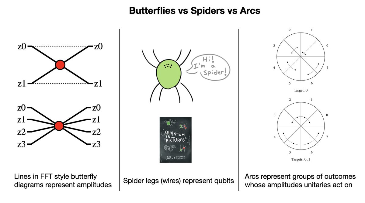
We can use state tables and polar (circular) representations, but we can also reference the "butterfly" diagrams used in the Fast Fourier Transform literature. In fact, the process of applying an elementary quantum gate is virtually the same as a stage in the (most common implementation of the) Fast Fourier Transform algorithm.
Each gate comes with its own formula, which is applied to all pairs of amplitudes.
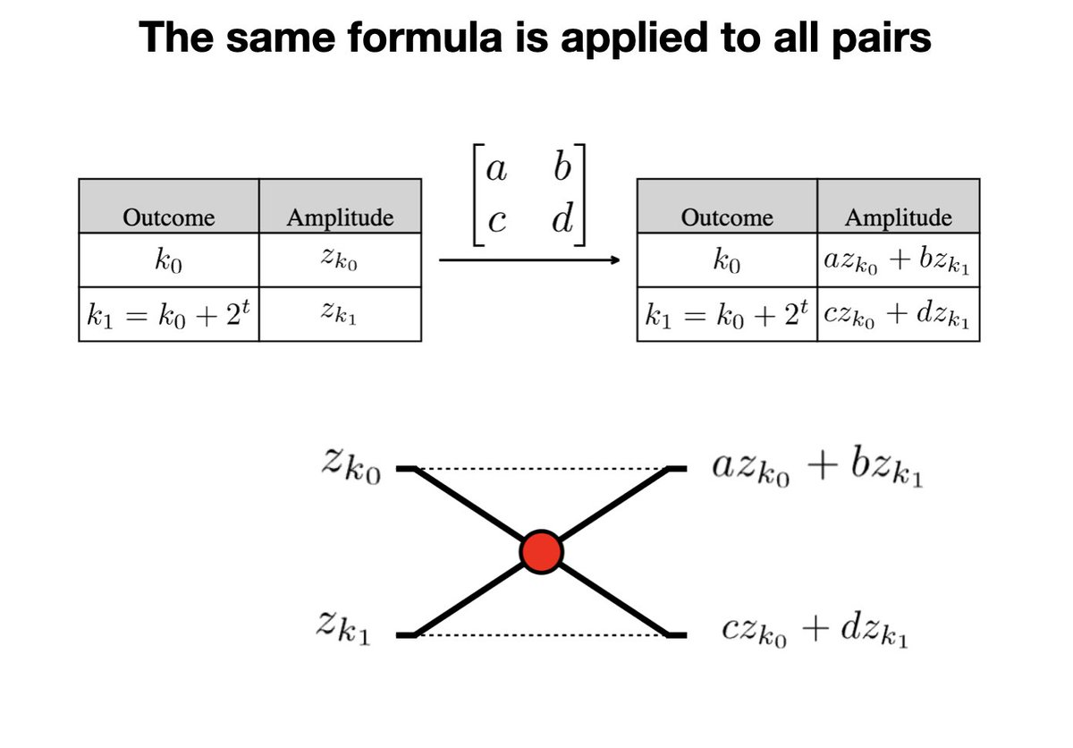
As an example, let's look at a visualization of the effect of applying the X-gate on qubit 0 of a three-qubit system. The amplitudes in each pair are swapped. For other gates, a different formula is applied to recombine the amplitudes in each pair, but the pairing mechanism is the same.
How to use this app: Select a gate, target qubit, and (if needed) a control qubit using the controls above the visualizer. Click 'Start Transformation' to begin the process - this will highlight the first pair of amplitudes that will be transformed. The pairs represent outcomes whose binary representations differ only in the target qubit position. For controlled gates, only pairs where the control qubit is 1 will be processed. Use 'Process Next Pair' to transform one pair at a time, or 'Process All Pairs' to complete the transformation at once. 'Reset' returns to the default state, and 'Randomize' creates a new random state. You can experiment with different gates and qubit choices to see their effects on the quantum state.
Try with target qubits 0, 1, and 2:
A gate-based quantum transformation applies a quantum gate to a target qubit and has a number of control qubits (different from the target). The same gate formula is used to process amplitude pairs, but only the paired outcomes that have 1 in the control positions get their amplitudes processed. For example, in a three-qubit system, if the middle qubit is a control qubit, the outcomes that have 0 as the middle digit in their binary representation are left unchanged. They are shown grayed out in the image that shows the pairs corresponding to target qubit 0. The paired outcomes differ only in the last digit (qubit 0).
Try different target and control qubits:
The behavior of quantum gates is a fascinating blend of the familiar and the unexpected. Just as we're accustomed to transfers between investments, quantum gates act similarly, transferring amplitudes (balances) between outcomes (accounts). However, here's where the twist lies: unlike in our everyday world, these "transfers" occur simultaneously, governed by the same mathematical formula. This is called quantum parallelism.
This simultaneous operation is the secret sauce of quantum computing, offering unparalleled advantages in certain applications. Yet, this very feature also restricts the types of problems that can benefit from a quantum approach.
These quantum mechanics concepts are crucial to the implementation of quantum computers, but are not directly relevant to quantum computing. Quantum superposition expresses the uncertainty of what outcome will be observed in a measurement. Quantum entanglement refers to the fact that individual qubit measurements are not always independent of each other. It is the implementation mechanism for controlled transformations.
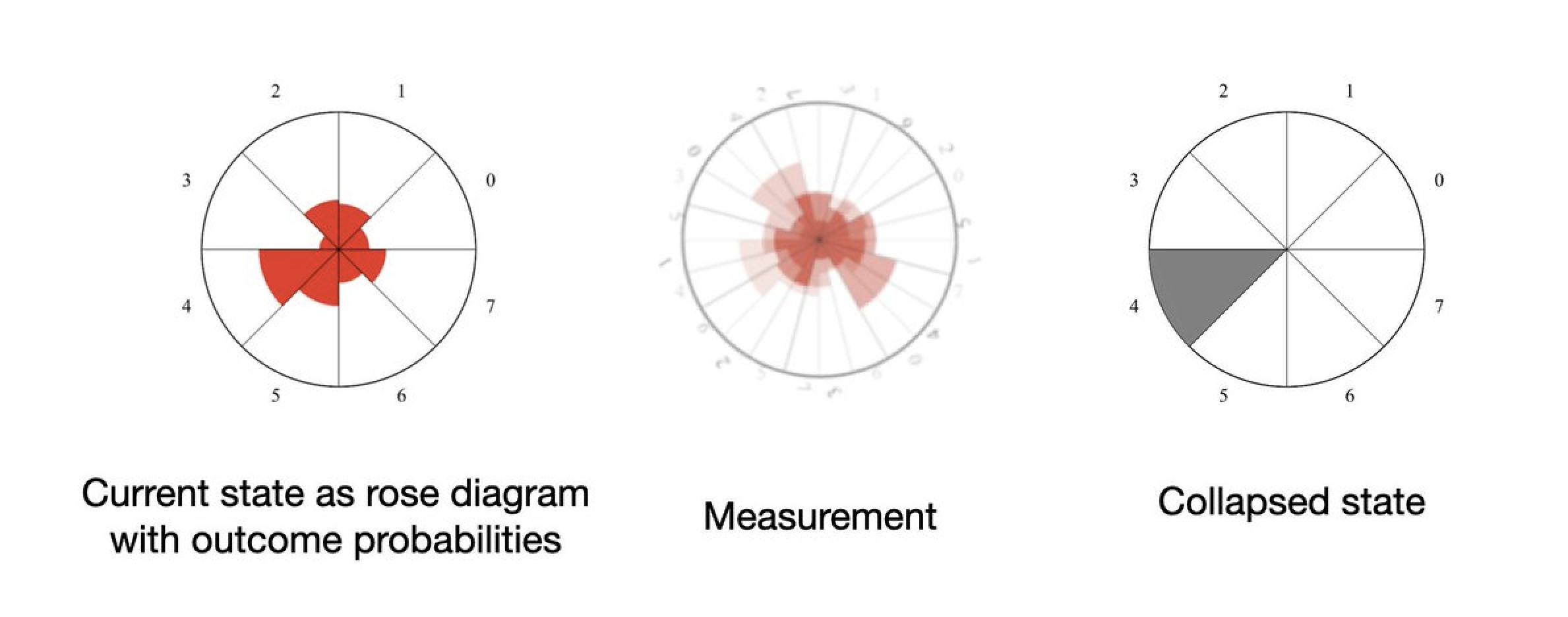
How can we visualize the measurement operation of a quantum state? In the measurement context, a quantum state is essentially a probability distribution. The probability of an outcome is the squared magnitude of its amplitude. Measurement is sampling from this probability distribution, and the measurement outcome is the sample. This outcome receives probability 1 after measurement. We visualize the state as a rose (polar area) diagram, which is the circular version of a bar chart, and the measurement as spinning this diagram. The resulting collapsed state is a rose diagram where the measurement outcome has probability 1 (and the rest of the outcomes have probability 0).
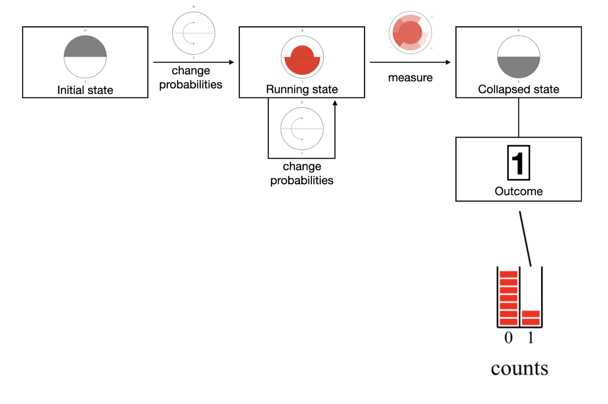
Putting the fundamentals together: start with the default quantum state, change it with quantum transformations, measure it, record the outcome and repeat.
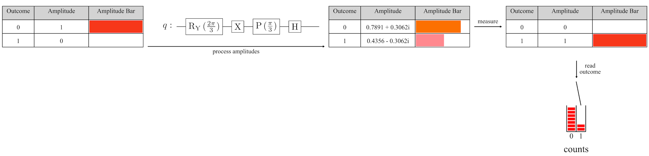
Here is an example of a one-qubit system evolution and measurement.
We can visualize the general case of running a one-qubit quantum computation as follows.
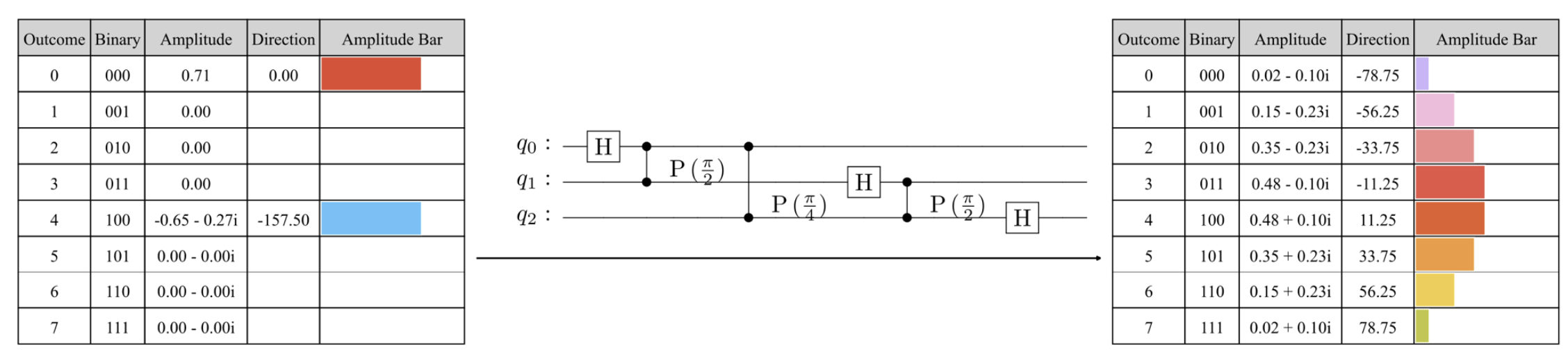
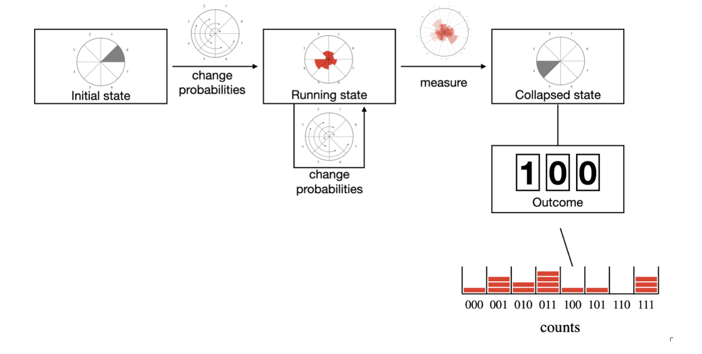
similarly, we can visualize the process of running a multi-qubit computation.
A quantum program, or circuit, consists of a sequence of quantum transformations. A typical transformation in a qubit-based quantum system is defined by a single-qubit gate, a target qubit, and a number of other control qubits.
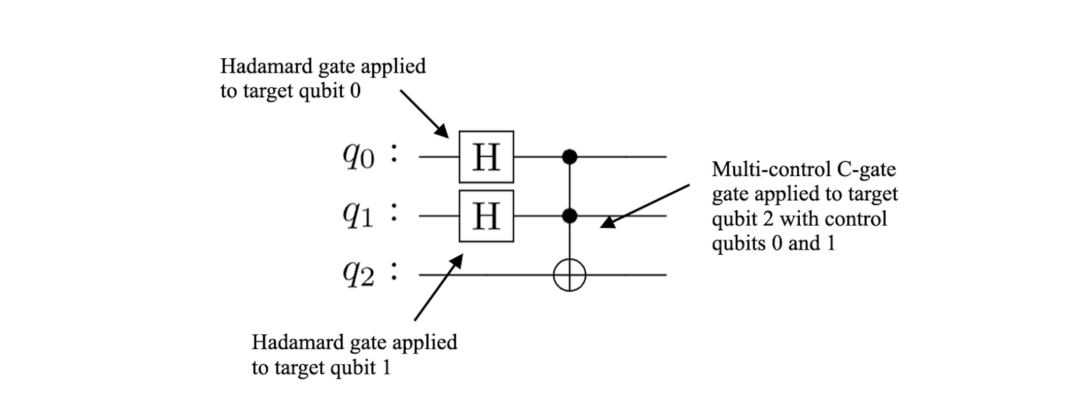
We can show circuits together with the states before and after their application.
Play around with a quantum circuit in your browser: Quantum Circuit
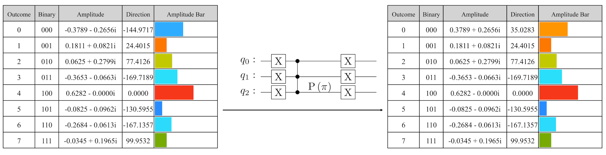
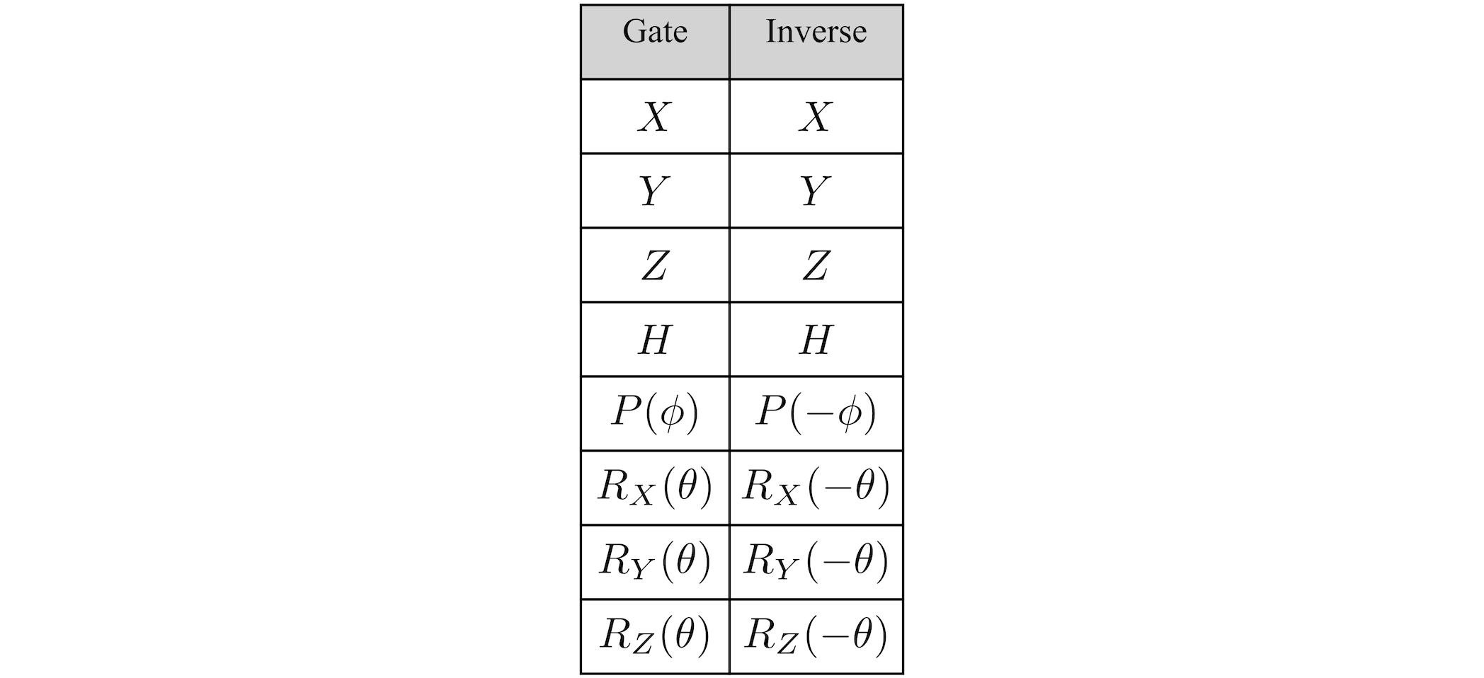
An important property of quantum transformations is that they are reversible: each has an inverse that cancels its action. The inverse of a transformation is obtained by using the inverse of its underlying elementary gate, and keeping the target and controls as they are.
The inverse of a circuit is obtained by applying the inverses of its transformations in reversed order.
Quantum advantage comes from exploiting quantum parallelism and measurement. In order to exploit parallelism, we need to counter its side effect: all amplitudes change in pairs according to a common formula. This is done through interference, where simultaneous changes to the numbers comprising a quantum state have to be balanced with the right types of changes. There are a few sources of useful natural interference, mostly present in the Phase Estimation and Amplitude Amplification algorithms. Since interference is hard, people try to find it using brute force search (variational algorithms). This is similar to finding weights for a neural network, but much more complex, hence the "brute force" term.
"The goal in devising an algorithm for a quantum computer is to choreograph a pattern of constructive and destructive interference so that for each wrong answer the contributions to its amplitude cancel each other out, whereas for the right answer the contributions reinforce each other. If, and only if, you can arrange that, you'll see the right answer with a large probability when you look."
-- Scott Aaronson, What Makes Quantum Computing So Hard to Explain? June 8, 2021, Quanta Magazine
Looking for quantum advantage is essentially looking for sources of interference.
Quantum computing is very specialized, and will not replace traditional computing, in the same way helicopters cannot replace cars. Quantum parallelism and quantum measurement can help solve problems that cannot easily be solved with classical computers, but at the same time they are not the right solution for most computing needs.
There are three main quantum computing patterns: sampling from probability distributions, searching for optimal values, and estimating the probability of certain computation outcomes. These patterns are described in more detail at learnqc.com.
The concepts introduced in this document give enough information to define the implementation of a simple quantum simulator. We include such a simple implementation in Appendix B, where we also include a simple test, and its equivalent in Qiskit, IBM's quantum framework. The same concepts have been used both in a learning version of a simulator, called Hume: https://github.com/learnqc/code, and a high-performance simulator written in Rust, called Spinoza: https://github.com/QuState/spinoza.
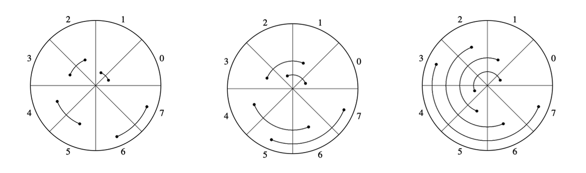
How do we visualize multi-target (sometimes called multi-qubit) transformations? We showed how single-qubit gates recombine pairs of amplitudes. It turns out that multi-target transformations process groups of amplitudes, and preserve the combined probability of each group. We can use the same type of visualization for the groups, where each group is represented by an arc, and each outcome belongs to exactly one group. The way the grouping is done depends on the target qubits. A single maximum size unitary processes all amplitudes as a group. While there are theoretical reasons to use such unitaries, most of the time we don't need to. It is more efficient to use a for loop to process the groups than to use a single giant unitary, and then rely on other tools to avoid multiplications by 0 and 1.
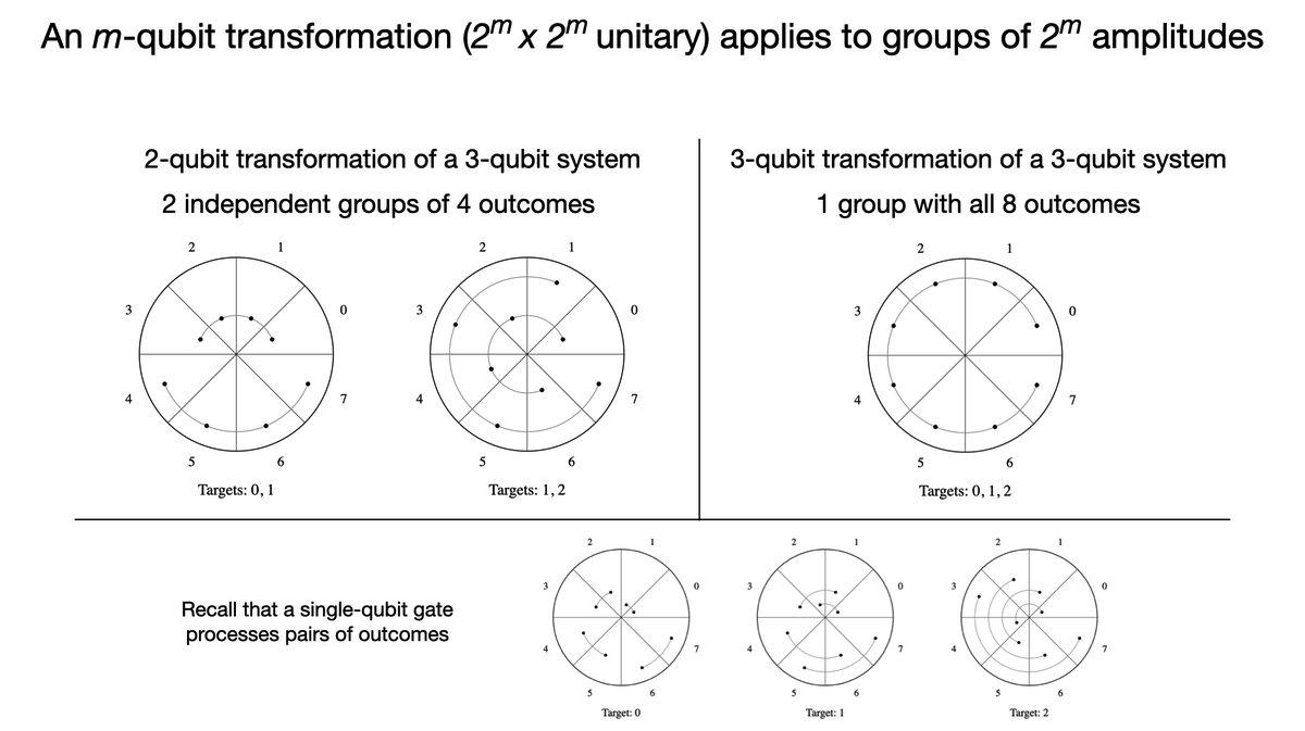
We can see that the arc diagrams have an advantage over the butterfly diagrams used in the Fast Fourier Transform literature. The arcs don't intersect, and they can capture all members of a group nicely.
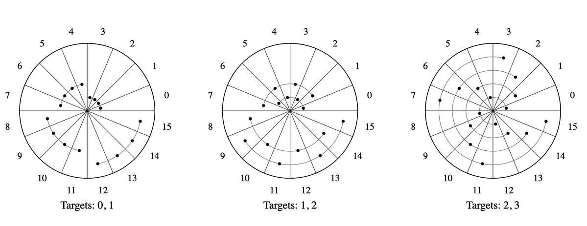
Also note that control qubits eliminate some groups from the processing. Only groups of outcomes having 1 as a binary digit in the control positions are processed. In a simulator, this significantly speeds up computations. On real computers, control qubits are expensive.
You may say: "The butterfly diagrams look more like spiders than butterflies". Indeed. The "butterfly" name is established in the Fast Fourier Transform literature. Butterfly diagrams show how complex numbers are recombined, while spider diagrams are wire diagrams that focus on qubits, with a complete formal theory behind them. Arc diagrams show the groups of outcomes whose amplitudes are transformed by a unitary.
  const x = [[0, 1], [1, 0]];
  const z = [[1, 0], [0, -1]];

  function phase(theta) {
    return [[1, 0], [0, math.complex(Math.cos(theta), Math.sin(theta))]];
  }

  const h = [[1 / Math.sqrt(2), 1 / Math.sqrt(2)], [1 / Math.sqrt(2), -1 / Math.sqrt(2)]];

  function rz(theta) {
    return [
      [math.complex(Math.cos(theta / 2), -Math.sin(theta / 2)), 0],
      [0, math.complex(Math.cos(theta / 2), Math.sin(theta / 2))]
    ];
  }

  const y = [[0, math.complex(0, -1)], [math.complex(0, 1), 0]];

  function rx(theta) {
    return [
      [Math.cos(theta / 2), math.complex(0, -Math.sin(theta / 2))],
      [math.complex(0, -Math.sin(theta / 2)), Math.cos(theta / 2)]
    ];
  }

  function ry(theta) {
    return [
      [Math.cos(theta / 2), -Math.sin(theta / 2)],
      [Math.sin(theta / 2), Math.cos(theta / 2)]
    ];
  }

  function initState(n) {
    const state = Array(2 ** n).fill(0);
    state[0] = 1;
    return state;
  }

  function isBitSet(m, k) {
    return (m & (1 << k)) !== 0;
  }

  function* pairGenerator(n, t) {
    const distance = 2 ** t;
    for (let j = 0; j < 2 ** (n - t - 1); j++) {
      for (let k0 = 2 * j * distance; k0 < (2 * j + 1) * distance; k0++) {
        const k1 = k0 + distance;
        yield [k0, k1];
      }
    }
  }

  function processPair(state, gate, k0, k1) {
    const x = state[k0];
    const y = state[k1];
    state[k0] = x * gate[0][0] + y * gate[0][1];
    state[k1] = x * gate[1][0] + y * gate[1][1];
  }

  function transform(state, t, gate) {
    const n = Math.log2(state.length);
    for (const [k0, k1] of pairGenerator(n, t)) {
      processPair(state, gate, k0, k1);
    }
  }

  function cTransform(state, c, t, gate) {
    const n = Math.log2(state.length);
    for (const [k0, k1] of pairGenerator(n, t)) {
      if (isBitSet(k0, c)) {
        processPair(state, gate, k0, k1);
      }
    }
  }

  function mcTransform(state, cs, t, gate) {
    const n = Math.log2(state.length);
    for (const [k0, k1] of pairGenerator(n, t)) {
      if (cs.every((c) => isBitSet(k0, c))) {
        processPair(state, gate, k0, k1);
      }
    }
  }

  function measure(state, shots) {
    const probabilities = state.map((amp) => Math.abs(amp) ** 2);
    const samples = math.pickRandom(state.map((_, i) => i), probabilities, shots);
    const counts = {};
    samples.forEach((sample) => {
      counts[sample] = (counts[sample] || 0) + 1;
    });
    return counts;
  }